Local Semantic Search: How On-Device AI Finds Meaning Without the Cloud

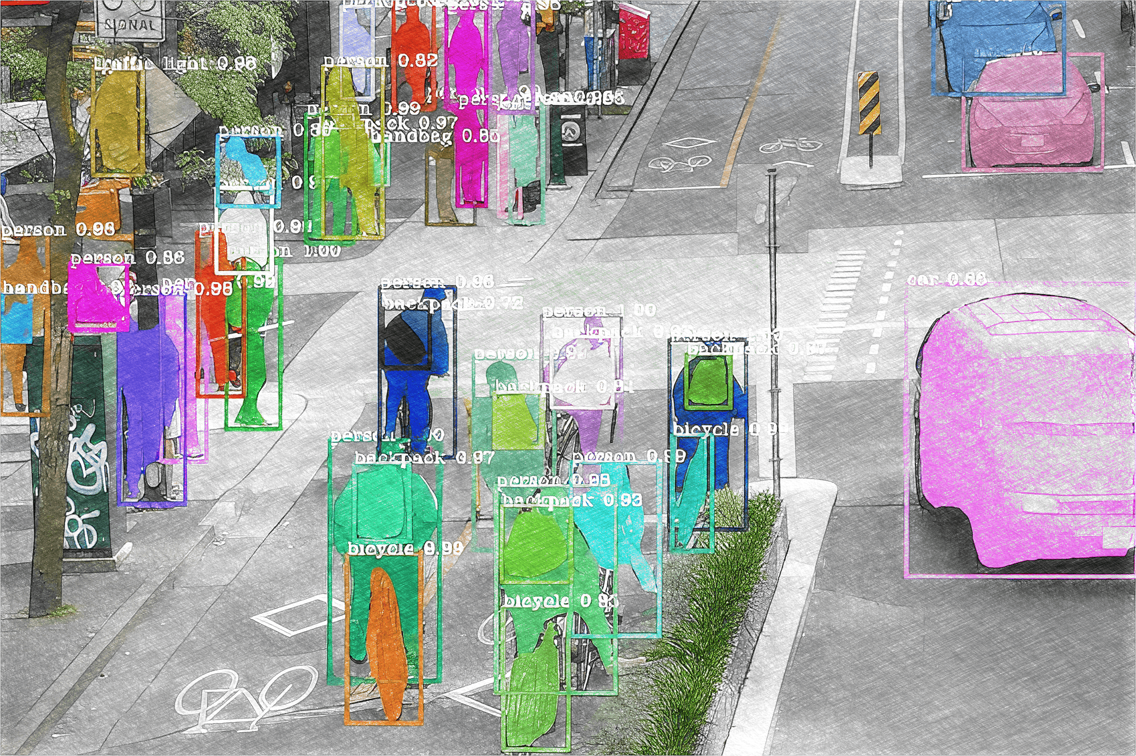
Search is the most fundamental interaction in computing, and for most of computing history it has been based on strings: you type a word, the system finds files whose names or contents contain that exact string. This works well when you know what the file is called. It fails completely when you remember what the file is about but not what it is named.

Semantic search solves this by understanding meaning. Instead of matching characters, it matches concepts. Type “dog on a beach” and it finds photos of dogs on beaches even if the filenames are IMG_4923.JPG. Type “Q4 budget proposal” and it finds documents about financial planning for the fourth quarter even if the files are named final_v3_revised_actual_final.docx.

The technology that makes this possible has existed in the cloud for years. The interesting development is that it now runs locally, on your own hardware, with no data leaving your machine. Here is how that actually works.

The Core Idea: Embeddings

At the heart of every semantic search system is an embedding model. An embedding model takes any input, a sentence, an image, an audio clip, and converts it into a fixed-length vector of floating-point numbers. A good embedding has the property that similar inputs produce similar vectors. The sentence “a golden retriever playing fetch” should be close in vector space to a photo of a golden retriever with a ball.

These vectors typically have 384 to 1536 dimensions. A 768-dimensional embedding from Nomic Embed Text v2, for example, is a point in 768-dimensional space. The position of that point encodes the semantic content of the input. Change the input meaning and the point moves. The geometry of the space maps to the semantics of the data.

Building a search index means running every file through the embedding model once and storing the resulting vectors. Searching means embedding the query and finding the stored vectors closest to it. The quality of the search depends entirely on the quality of the embedding model. If the model cannot distinguish between semantically different inputs, the search will not work.

The Math: Cosine Similarity and ANN

Comparing two embeddings requires a similarity metric. The standard choice is cosine similarity, which measures the angle between two vectors regardless of their magnitude:

cos(θ) = (A · B) / (||A|| * ||B||)

Where A · B is the dot product and ||A|| is the Euclidean norm. Cosine similarity ranges from -1 (opposite direction, opposite meaning) to 1 (same direction, same meaning). In practice, most embedding models produce vectors with positive cosine similarities for related content and near-zero similarities for unrelated content. When embeddings are L2-normalized to unit length, cosine similarity simplifies to the dot product, a single multiply-accumulate operation per dimension.

For a small index (thousands of vectors), brute-force search is acceptable: compute the cosine similarity between the query and every stored vector, then take the top-k results. The complexity is O(n*d) where n is the number of vectors and d is the dimensionality. For hundreds of thousands or millions of vectors, brute force becomes too slow. This is where approximate nearest neighbor (ANN) algorithms come in.

The most popular ANN algorithm for local semantic search is HNSW (Hierarchical Navigable Small World). HNSW builds a multi-layer graph: the top layer contains a small subset of nodes with long-range connections; each lower layer adds more nodes with shorter connections. Search starts at the top layer and greedily navigates to the nearest neighbor, then descends to the next layer and repeats. The result is O(log n) search complexity with recall above 99% in practice. Other approaches include IVF-PQ (inverted file indexing with product quantization) and locality-sensitive hashing (LSH), but HNSW dominates local deployment because it does not require training and works well on CPU.

Trending Local Models in 2026

The embedding model landscape has matured rapidly. In 2025 and 2026, several models have emerged as leaders for local deployment:

Nomic Embed Text v2. At 768 dimensions with 137M parameters, this model beats OpenAI’s text-embedding-3-small on the MTEB benchmark while being small enough to run on a laptop CPU. It uses Matryoshka Representation Learning, meaning the model produces embeddings that remain useful even when truncated to lower dimensions. A user can store 256-dimensional vectors for speed while retaining the option to use the full 768 dimensions for high-precision queries.

BGE-M3 by BAAI. This model supports three retrieval paradigms in one architecture: dense embeddings (standard vector search), sparse embeddings (lexical matching like BM25), and multi-vector retrieval (ColBERT-style late interaction). It handles multilingual content across 100+ languages and supports document lengths up to 8192 tokens. The small variant at 102M parameters runs comfortably on device.

GTE-Qwen2 by Alibaba. Built on the Qwen2 language model, GTE-Qwen2 achieves state-of-the-art results on Chinese and English retrieval benchmarks. The 1.5B parameter version is too large for most local deployments, but Alibaba released distilled variants at 300M and 100M parameters that retain most of the retrieval quality.

Snowflake Arctic Embed L. Optimized specifically for retrieval quality rather than general-purpose embeddings, Arctic Embed L uses a two-stage training pipeline: first contrastive learning on mined pairs, then hard-negative mining with a teacher model. At 1.5B parameters, it is best suited for desktop deployment with GPU acceleration, but quantized 4-bit versions bring it to 900 MB of memory.

CLIP and its variants. For multimodal search (text-to-image, image-to-image), OpenAI’s CLIP and its open successors like SigLIP and DFN remain the standard. These models use dual encoders: one transformer for text, one vision transformer for images, projected into a shared embedding space. The ViT-B variant has 86M vision parameters and 63M text parameters, small enough to run on a modern laptop with ONNX Runtime.

Optimization: Making Models Fit on Everyday Devices

Running a neural network on a laptop or phone requires aggressive optimization. Here are the techniques that make local semantic search practical:

Quantization. A model’s weights are normally stored as 32-bit floating-point numbers (4 bytes each). Quantization reduces each weight to 8-bit integers (1 byte) or 4-bit integers (0.5 bytes), shrinking the model by 4x to 8x. Post-training quantization (PTQ) applies this conversion after training with a small calibration dataset; quantization-aware training (QAT) simulates quantization during training and produces higher-quality results. For embedding models, 4-bit quantization typically reduces MTEB scores by less than 1% while cutting memory from gigabytes to megabytes.

Knowledge Distillation. A large teacher model (e.g., 1.5B parameters) trains a smaller student model (e.g., 100M parameters) to reproduce its outputs. The student learns to match the teacher’s embedding vectors on a diverse training corpus, then replaces the teacher at inference time. This is how models like GTE-Qwen2 produce their 100M-parameter variants.

ONNX Runtime. Microsoft’s cross-platform inference engine is the backbone of most local AI deployment. ONNX Runtime applies operator fusion (combining multiple operations into a single kernel), memory optimization (reusing buffers, eliminating copies), and hardware-specific execution providers (DirectML on Windows, CoreML on macOS, OpenVINO on Intel, TensorRT on NVIDIA). A model running through ONNX Runtime can be 2-5x faster than the same model in raw PyTorch.

Progressive Filtering. For image search, a common optimization is progressive filtering: run a cheap embedding model first to narrow candidates, then run a more expensive model on the survivors. A typical pipeline might use a 50M-parameter model for initial retrieval of the top 500 results, then re-rank with a 300M-parameter model. This provides near-top-tier accuracy at a fraction of the compute cost.

Why Local Matters

Running semantic search locally is not just about latency or cost. It is about privacy. When search runs on your device, your files never leave your machine. No cloud upload, no training on your data, no exposure to server breaches. For businesses handling confidential documents, legal files, or proprietary design assets, this is not a nice-to-have; it is a requirement.

It is also about reliability. Cloud search stops working when your internet drops, when the API provider changes pricing, or when the service is deprecated. Local search works the same way every time, regardless of network conditions.

The models have reached the point where the trade-off between quality and locality is negligible. A quantized Nomic Embed Text v2 running on a laptop CPU achieves within striking distance of cloud-hosted models twice its size. The gap will close further, and possibly reverse, as hardware accelerators become standard in consumer devices.

What This Actually Means

Local semantic search has crossed the threshold from demo to product. The models are good enough, the optimizations are mature enough, and the hardware is capable enough that searching files by meaning rather than by name is practical on any reasonably modern laptop. The remaining work is in user experience: making semantic search feel as natural and reliable as string search, while preserving the privacy and offline capabilities that local deployment provides.

For anyone building a local search product, the starting point in 2026 is clear: use Nomic Embed Text v2 or BGE-M3 for text, CLIP or SigLIP for images, ONNX Runtime for inference, and HNSW for vector search. Quantize to 4-bit, index once, and search at the speed of thought. The math might be complex, but the result is simple: find what you need, without saying what it is called.